Overview of Agricultural Indices
This section contains a quick discussion on the main vegetation indices used in agricultural-related remote sensing. Below contains a summary of each index,
the formula and what it is used for.
For the uninitiated and those wanting a little context, I begin with a super simple intro to sensors and multispectral imaging.
What use is aerial imagery for agriculture?
Aerial photos can be used for crop scouting. Rather than having to walk fields an aerial view can be used to determine the status of the crop. After planting aerial
images can be used to determine if the crop is established.
Once growth is underway photos can be used to determine crop density or crop health, sometimes with the latter, the use of multispectral
sensors detailing invisible light in the near infrared can give an early indication of health before problems become apparent to the naked eye.
Based on feedback from aerial surveys fertilzer prescriptions can be developed whereby the map of the field is used to apply fertilizer just to those areas of the crop that require it,
thus saving on expenditure for fertilzer and fuel.
Machine learning can be used to calculate plant counts rapidly over a large area. This can be useful for estimating likely yield. This would typically be for vegetables or trees.
Depending on the locale, video or true colour imagery can be used for insurance claims should crops be damaged.
A Quick Intro to Multispectral Imaging
We can use aerial and satellite images to monitor the Earth's surface. These are often referred to as "sensors" and are effectively the same technology as found in modern day cameras, in fact the digital camera has its
origins in sensors developed for use in satellite photography - one of the earliest being in 1972 and used in Landsat 1's multispectral scanner here.
Digital cameras work by capturing light reflected off different surfaces (could be your cat or the Earth). Light is a wave (sometimes!) and is known as the electromagnetic spectrum, some of this we can see and some we cannot.
Visible light is the rainbow of colous which can be made up from Red, Green and Blue. Invisible light includes microwaves and infrared. The sensors on satellites, and some cameras, capture not only visible but also this invisible light
(for example with thermal cameras).
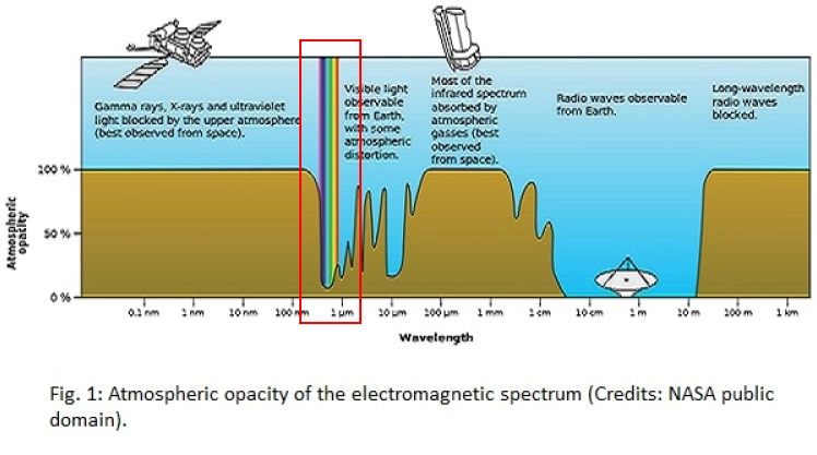
Satellites and aerial photos measure the reflectance of light in different bands (e.g. Red, Green, Blue, Infrared etc.) which represent different wavelengths (energies) of light. Satellites are very useful as they
can survey a wide area but they can be affected by cloud cover and atmospheric haze. Further, only certain wavelenghts of light will be obvservable from space due to atmospheric absorption. Aerial photos, especially from low flying drones,
get around most of these limitations. Drones also have a much higher resolution that satellites providing images where each pixel is centimetre or sub-centimetre level whereas most free satellite images are 10+ metres
(sub-metre resolution is available from paid-for service providers although these tend to be expensive).
A further advantage of drones is that they can be deployed as required whereas satellite images are only available on rotation when the satellite is overhead (known as the return period). This can vary from a few days to weeks. The images
provided further below in this article are from the Sentinel 2 satellite which has a resolution of 10m and a return period of around 10 days depending on latitude.
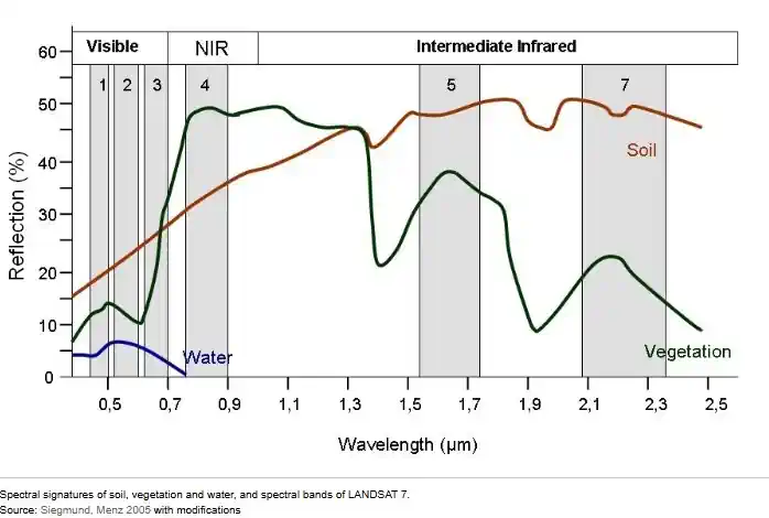
Different materials reflect different levels of light. Black objects reflect little light (hence being black) whereas white objects would reflect all (most) visible light. Figure 2 below shows the differences in reflectivity
of water, vegetation and soil. We can see that each material reflects light in different bands (at different wavelengths). The numbered bands in figure 2 are the wavelengths that are captured by the Landsat 7
satellite (1,2,3 being blue, green, red and 4 being near infrared). The sensors on satellites have been specifical chosen/designed to target wavelengths that are of interest and will vary between satellites depending on the
objective of the system. The Landsat satellite was specifically designed to explore environmental matters and hence having sensitivity in this region for detecting vegetation.
We can see that for vegetation there is very little reflectance in bands 1-3 (visible light from 400 to 700 nm). This is because the visible light in is absorbed in the process of
photosynthesis. We also see a big spike in reflected light from (from 700 to 1100 nm). This is known as the "red edge" and is due to
light being reflected from the cell structure in leaves in the near infrared wavelength.
When plants are healthy, they have a high chlorophyll content, which allows them to absorb more light in the red region of the spectrum and reflect more light in the NIR region.
Conversely, if there is less chlorophyl in the plant then more light will be reflected in the visible spectrum.
Multispectral sensors give us the ability to examine the non-visible light reflected from vegetation and this can be a good indicator of crop health. Be this the density of the crop, the canopy depth or
it could actually give us a window into weeds rather than the target crop itself. Other wavelengths allow us to examine water in the crop or soil. These are touched on below.
Indices Summary and Calculations
| Index | Calculation | Comment |
|---|---|---|
| NDVI | (NIR – red) / (NIR + red) | Normalised Difference Vegetation Index |
| GNDVI | (NIR - GREEN) / (NIR + GREEN) |
Green Normalized Difference Vegetation GNDVI is more sensitive to chlorophyll variation in the crop than NDVI and has a higher saturation point. |
| NDRE | (NIR – RED EDGE) / (NIR + RED EDGE) |
Normalized Difference Red Edge can detect variations in crop health at more advanced stages. with a more intense canopy, it is advisable to use NDRE because NDVI saturates. |
| MSAVI2 | see image to right |
Modified Soil Adjusted Vegetation Index. variant to extend the application limits of NDVI to areas with a high presence of bare soil. Minimizes the influence of the soil
background and increases the dynamic range signaled by the vegetation.
It minimizes bare soil’s influence, so it is ideal for early stages, such as crop emergence, crops that do not cover the soil in its most developed stage, or woody crops. 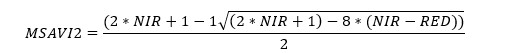
|
| NDWI | (NIR-SWIR) / (NIR+SWIR) |
Normalized Difference Water Index. Used to monitor crop water status. As with other indices,
the values obtained for NDWI range from -1 to 1, where high values correspond to high plant water content. |
| SAVI |
((NIR - Red) / (NIR + Red + L)) * (1 + L) |
Soil Adjusted Vegetation Index. L is the soil adjustment factor and is crucial for SAVI's effectiveness. It's typically set to 0.5 for areas with moderate vegetation cover. In areas with very high vegetation cover, L approaches 0, making SAVI similar to NDVI. Conversely, in areas with very low vegetation cover, L approaches 1. Mitigate the impact of soil on spectral measurements and enabling more reliable analysis of vegetation cover, particularly in areas where soil is visible. https://www.sciencedirect.com/science/article/abs/pii/0034425794901341 |
NDVI
The Normalised Difference Vegetation Index (NDVI) is by far the most common index used to evaluate crop coverage. It is expressed as a ratio between the difference in reflectance of near infrared
and red bands over the sum of these values. This presents a normalised figure ranging from -1 to 1.
In general, if there is much more reflected radiation in near-infrared wavelengths than in visible wavelengths, then the vegetation in that pixel is likely to be dense. Dense vegetation would have
a value in the region of 0.3 - 1. Negative values would indicate a lack of vegetation. Some sources indicate a classification / interpretation as below, although this would vary from
crop to crop and the point in the growth cycle. In reality the index is linear and therefore strict classification is perhaps not helpful, rather we should be exploring differences and
seeking to understand what is happening in those locations.
| -1 | 0 | No vegetation |
| 0 | 0.33 | Unhealthy/sparse vegetation |
| 0.33 | 0.66 | Moderately healthy / dense vegetation |
| 0.66 | 1 | Healthy / very dense vegetation |
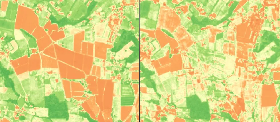
Figures 3 and 4 below show ndvi and true colour images using Sentinel 2 satellite data. The image on the left in each instance is from September 2024 and on the right is from June 2025. In figure 4, we can clearly see that some areas have been ploughed and are bare soil (sept - left image) whereas the fields are planted with crops come June (right image). This difference is relfected in the ndvi images. We can see that the ploughed areas appear red whereas the planted areas appear green. These red areas have an ndvi value of around 0 - 0.2 so don't quite fit the classification above, however as noted it is the difference rather than the specific value that is of use.
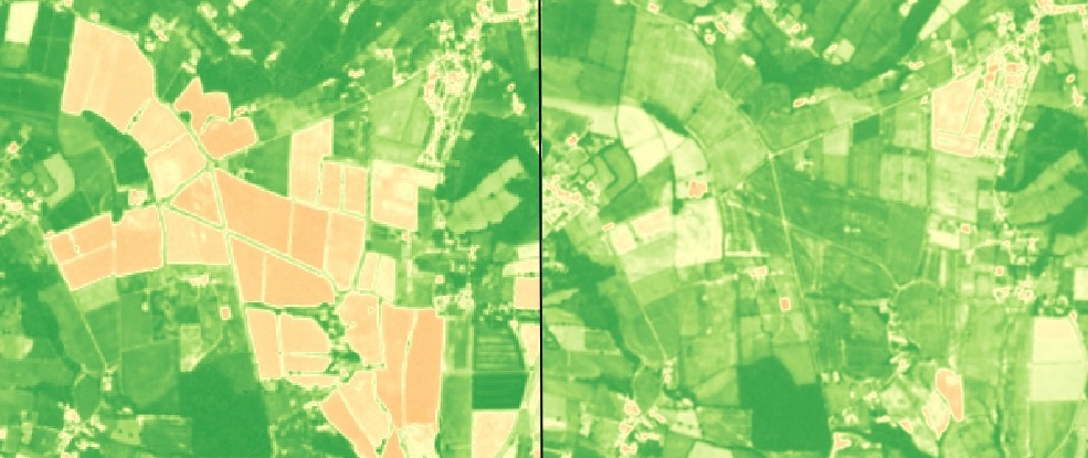
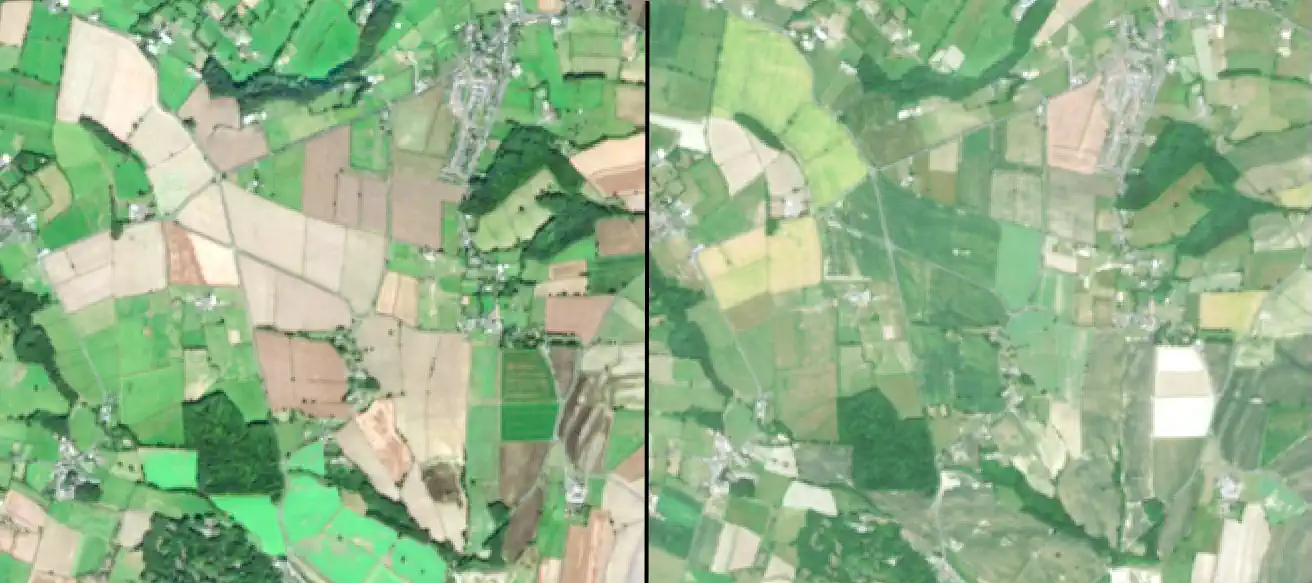
The satellite imagery used in these examples is of quite low resolution in these example, each pixel representing 10 metres on the ground. This is fine for scientists wanting to undertake studies of land cover over a very wide area but
is very limiting for smaller fields. It doesn't offer much by way of insight. Using a drone with centimetre level resolution is where one can really start to get actionable insights that could
be of value to a farmer. See the example in banner at the top of this article for a higher resolution example captured by drone.
NDVI can become saturated whereby there is limited difference between the values and therefore we get reduced useful information. One way to address this is to improve the classification (i.e. using a colour ramp with a wide range of colours)
or we can look to some of the other indices that have been specifically designed to counter issues of saturation.
Sources
Precision agricultire - Wikipedia
Red Edge - Wikipedia
NDVI - Wikipedia
NDRE - Wikipedia
NDWI - Wikipedia
NDVI - discussion on cropin website
Indices discussion on auravent.com
How to make an NDVI in QGIS
NDVI intro (auravant site)
Tools and Software
Auravant (Digital Agriculture Platform)Cropin (Digital Agriculture Platform)